Basic Usage of the tyssue library

Easy creation of a 2D epithelial sheet

In tyssue, an apical junction network is represented as a mesh. The structure of this mesh is stored in three tables (pandas.DataFrame objects) corresponding to vertices, faces and edges. The structure and data associated with these meshes are detailed bellow.

%matplotlib inline

# Core object
from tyssue import Sheet
# Simple 2D geometry
from tyssue import PlanarGeometry as geom
# Visualisation
from tyssue.draw import sheet_view

sheet = Sheet.planar_sheet_2d(
    'basic2D', # a name or identifier for this sheet
    nx=6, # approximate number of cells on the x axis
    ny=7, # approximate number of cells along the y axis
    distx=1, # distance between 2 cells along x
    disty=1 # distance between 2 cells along y
)
geom.update_all(sheet)

This module needs ipyvolume to work.
You can install it with:
$ conda install -c conda-forge ipyvolume

CGAL-based mesh generation utilities not found, you may need to install CGAL and build from source
C++ extensions are not available for this version

The sheet_view function displays the created object in a matplotlib figure:

fig, ax = sheet_view(sheet)
fig.set_size_inches(8, 8)

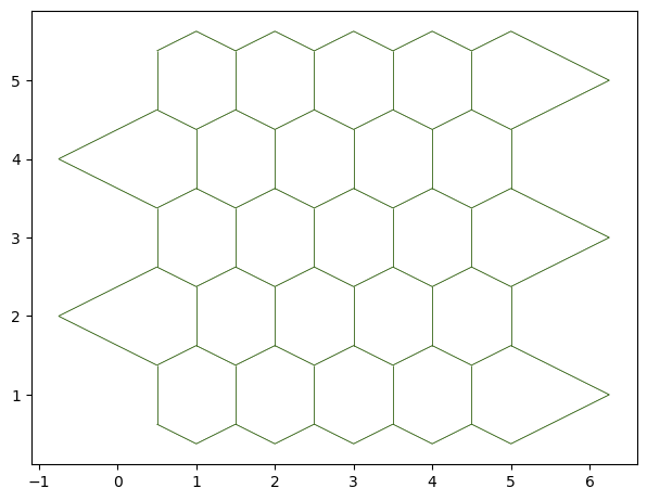
We can have a cleaner, better ordered sheet with the sanitize method:

# Give the tissue a nice hear cut ;)
sheet.sanitize(trim_borders=True, order_edges=True)
geom.update_all(sheet)

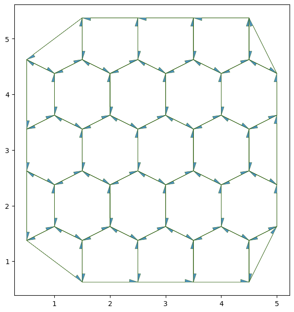
Here we pass an option to display the edge directions see the visualization tutorial for details

fig, ax = sheet_view(
    sheet, 
    mode="2D",
    edge={"head_width": 0.1}
)
fig.set_size_inches(8, 8)

You can look at the tyssue.generation module for more sheet creation utilities.

A remark on the half-edge data structure

As is represented in the above graph, each edge between two cells is composed of two half-edges (only one half-edge is present in the border ones). This makes it easier to compute many cell-specific quantities, as well as keeping a well oriented mesh. This is inspired by CGAL polyhedral surfaces.

Datasets

The data associated with the mesh displayed above, i.e. the points positions, the connectivity information, etc. is stored in pandas DataFrame objects, hold together in the datasets dictionnary.

Depending on the geometry, the following dataframes are populated:

• datasets["edge"] or sheet.edge_df: The edge related dataframe contains the connectivity information: source and target vertices, associated face and (for thick tissues) the associated cell body, geometry data associated with the edge, such as its length and any suplemental data, such as a color or a dynamical parameter (an elasticity for example)

• datasets["vert"] or sheet.vert_df: The vertices related dataframe. In the apical junction mesh above, those are the vertices at the cells junctions. It usually holds the coordinates of the points, and geometry or dynamical data.

• datasets["face"] or sheet.face_df: The faces related dataframe. For a thin, 2D tissue, this corresponds to a cell of the epithelium, delimited by its edges. In thick, 3D models, one cell has several faces (the apical, sagittal and basal ones for a 3D monolayer, for example).

• datasets["cell"] or sheet.cell_df: The cells related dataframe, only for 3D, thick, epithelium. Each cell have several faces.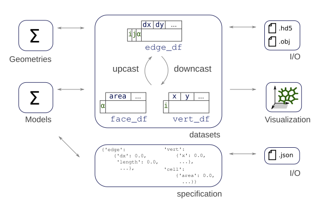

  

for element, data in sheet.datasets.items():
    print(f"{element} table has shape {data.shape}")

vert table has shape (48, 3)
edge table has shape (128, 20)
face table has shape (25, 7)

sheet.datasets['edge'].head()

	trgt	nz	length	face	srce	dx	dy	sx	sy	tx	ty	fx	fy	ux	uy	rx	ry	sub_area	is_valid	phi
edge
0	30	0.28125	0.750000	0	28	0.0	0.75	1.5	0.625	1.5	1.375	1.125	1.250	0.000000	1.000000	0.375	-0.625	0.140625	True	-0.643501
1	9	0.15625	0.559017	0	30	-0.5	0.25	1.5	1.375	1.0	1.625	1.125	1.250	-0.894427	0.447214	0.375	0.125	0.078125	True	0.643501
2	5	0.21875	0.559017	0	9	-0.5	-0.25	1.0	1.625	0.5	1.375	1.125	1.250	-0.894427	-0.447214	-0.125	0.375	0.109375	True	1.570796
3	28	0.34375	1.250000	0	5	1.0	-0.75	0.5	1.375	1.5	0.625	1.125	1.250	1.788854	-1.341641	-0.625	0.125	0.171875	True	1.570796
4	43	0.37500	0.750000	1	29	0.0	0.75	2.5	0.625	2.5	1.375	2.000	1.125	0.000000	1.000000	0.500	-0.500	0.187500	True	-0.643501

The edge_df dataframe contains most of the information. In particular, each time the geometry is updated with the geom.update_all(sheet) function, the positions of the source and target vertices of each edge are copied to the "sx", "sy" and "tx", "ty" columns, respectively.

sheet.face_df.head()

	y	is_alive	perimeter	area	x	num_sides	id
face
0	1.250000	1	3.118034	0.5000	1.125000	4	0
1	1.125000	1	3.618034	0.8750	2.000000	5	0
2	1.125000	1	3.618034	0.8750	3.000000	5	0
3	1.125000	1	3.618034	0.8750	4.000000	5	0
4	1.208333	1	2.427051	0.1875	4.666667	3	0

We can use all the goodies from pandas DataFrames objects. For example, it is possible to compute the average edge length for each face like so:

sheet.edge_df.groupby('face')['length'].mean().head()

face
0    0.779508
1    0.723607
2    0.723607
3    0.723607
4    0.809017
Name: length, dtype: float64

Specifications

Specifications are defined as a nested dictionnary, sheet.specs. For each element ("vert", "edge", face", "cell"), the specification defines the columns of the corresponding DataFrame and their default values. An extra key at the root of the specification is called "settings", and can hold specific parameters, for example the arguments for an energy minimization procedure. For exemple, consider the following spec dictionnary

spec = {
    "vert": {
        "x": 0.0,
        "y": 0.0,
        "active": True
    },
    "edge": {
        "tension": 0.0,
        "length": 1,
    },
    "face": {
        "area": 0.0,
        "alive": True,
    },
}

This defines e.g an "area" column for sheet.face_df.

By calling sheet.update_specs(specs) method, those columns will be added to the respective dataframes.

sheet.update_specs({"edge": {"tension": 0.0}})
sheet.edge_df['tension'].head()

edge
0    0.0
1    0.0
2    0.0
3    0.0
4    0.0
Name: tension, dtype: float64

Optionaly, you can pass reset=True to update_spec (a warning is emitted):

sheet.update_specs(
    {"edge": {"tension": 1.0}},
    reset=True
)
sheet.edge_df['tension'].head()

edge
0    1.0
1    1.0
2    1.0
3    1.0
4    1.0
Name: tension, dtype: float64

Input and Output

The ‘native’ format is to save the datasets to hdf5 via pandas.HDFStore. The io.obj also provides functions to export the junction mesh or triangulations to the wavefront OBJ format (requires vispy), for easy import in 3D software such as Blender.

Here is the code to save the data in wavefront OBJ:

obj.save_junction_mesh('junctions.obj', sheet)

The standard data format for the datasets is HDF:

from tyssue.io import hdf5

Writing

hdf5.save_datasets('tmp_data.hdf5', sheet)

Reading

dsets = hdf5.load_datasets('tmp_data.hdf5')
sheet2 = Sheet('reloaded', dsets)

!rm tmp_data.hdf5

Specs can be saved as json files:

import json

with open("tmp_specs.json", "w") as jh:
    json.dump(sheet.specs, jh)

And reloaded accordingly

with open("tmp_specs.json", "r") as jh:
    specs = json.load(jh)

sheet2.update_specs(specs, reset=False)

!rm tmp_specs.json

This should evolve in the future to have a “single shop stop” for all the data, surely as a zarr data store. Also we plan on using meshio as an I/O interface.

Upcasting and downcasting data

It is often necessary to use a vertex-associated data on a computation involving faces, are other combinations of elements. Tyssue offers the upcast and downcast mechanisms to do that.

This part is less important for an immediate use of tyssue, you can skip it at first.

Upcasting

Geometry or physics computations often require to access for example the cell related data on each of the cell’s edges. The Epithelium class and its derivatives defines utilities to make this, i.e copying the area of each face to each of its edges:

print('Faces associated with the first edges:')
print(sheet.edge_df['face'].head())
print('\n')

# First edge associated face
face = sheet.edge_df.loc[0, 'face']

print('Area of cell # {}:'.format(int(face)))
print(sheet.face_df.loc[face, 'area'])

print('\n')
print('Upcasted areas over the edges:')
print(sheet.upcast_face(sheet.face_df['area']).head())

Faces associated with the first edges:
edge
0    0
1    0
2    0
3    0
4    1
Name: face, dtype: int64


Area of cell # 0:
0.5


Upcasted areas over the edges:
edge
0    0.500
1    0.500
2    0.500
3    0.500
4    0.875
Name: area, dtype: float64

The values have indeed been upcasted. This can also be done with the source and target vertices (sheet.upcast_srce, sheet.upcast_trgt) and cells in the 3D case (sheet.upcast_cell).

Downcasting

This is usually done by groupby operations as shown above. Syntactic sugar is available for summation, e.g. over every edges with a given source:

sheet.sum_srce(sheet.edge_df['tension']).head()

	tension
srce
0	3.0
1	2.0
2	2.0
3	3.0
4	3.0