import matplotlib.pyplot as plt
%matplotlib inline
import pandas as pd
import numpy as np

from tyssue import Sheet
from tyssue import PlanarGeometry
from tyssue.generation import generate_ring
from tyssue import config
from tyssue.draw import sheet_view

/tmp/ipykernel_3457/2882594318.py:3: DeprecationWarning: 
Pyarrow will become a required dependency of pandas in the next major release of pandas (pandas 3.0),
(to allow more performant data types, such as the Arrow string type, and better interoperability with other libraries)
but was not found to be installed on your system.
If this would cause problems for you,
please provide us feedback at https://github.com/pandas-dev/pandas/issues/54466
        
  import pandas as pd

CGAL-based mesh generation utilities not found, you may need to install CGAL and build from source
C++ extensions are not available for this version

This module needs ipyvolume to work.
You can install it with:
$ conda install -c conda-forge ipyvolume

Geometry classes

A Geometry class is a stateless class holding functions to compute geometrical aspects of an epithelium, such as the edge lengths or the cells volume. As they are classes, inheritance can be used to define more and more specialized geometries.

For the user, a geometry class is expected to have an update_all method that takes an Epithelium instance as sole argument.

Calling this method will compute the relevant geometry on the epithelium.

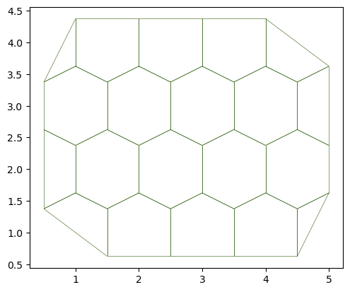
2D Geometries

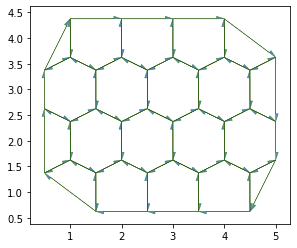
sheet_2d = Sheet.planar_sheet_2d('planar', nx=6, ny=6, 
                                 distx=1, disty=1)
sheet_2d.sanitize(trim_borders=True, order_edges=True)
fig, ax = sheet_view(sheet_2d)

Displacing vertices

Most of the geometry is purely defined by the vertex positions. It is possible to change those by modifying directly the vertex dataframe

For exemple, we can center the vertices around 0 like so:

com = sheet_2d.vert_df[sheet_2d.coords].mean(axis=0)
print("Sheet center of mass :")
print(com)

# Translate vertices by - 

sheet_2d.vert_df[sheet_2d.coords] -= com

print("New center of mass :")
print(sheet_2d.vert_df[sheet_2d.coords].mean(axis=0))

Sheet center of mass :
x    2.75
y    2.50
dtype: float64
New center of mass :
x    0.0
y    0.0
dtype: float64

The view does not change though:

fig, ax = sheet_view(sheet_2d)

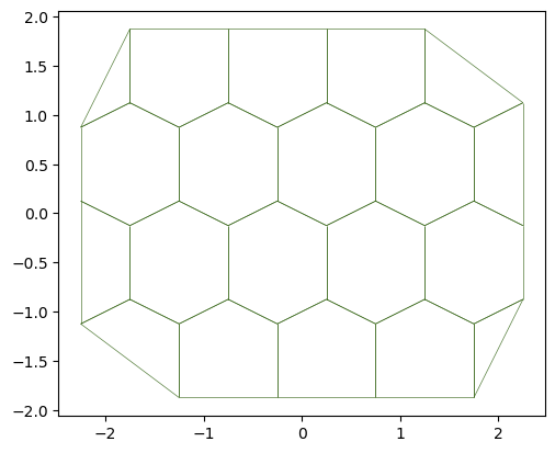
In order to propagate the change in vertex positions, we need to update the geometry:

PlanarGeometry.update_all(sheet_2d)

Now the sheet is centered:

fig, ax = sheet_view(sheet_2d)

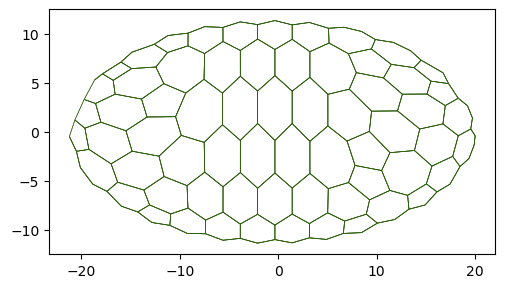
Closed 2D geometry

We can also use the generate_ring function to create a 2D ring of 4-sided cells.

ring = generate_ring(Nf=24, R_in=12, R_out=14)
PlanarGeometry.update_all(ring)

fig, ax = sheet_view(ring)

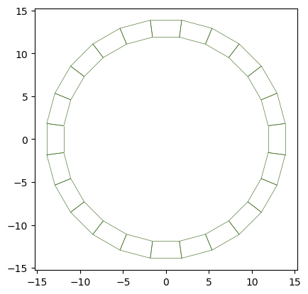
There is an AnnularGeometry class that does all PlanarGeometry does plus computing the “lumen” volume, here the area inside the ring.

from tyssue.geometry.planar_geometry import AnnularGeometry

AnnularGeometry.update_all(ring)
print(ring.settings["lumen_volume"])

894.4786198743117

Sheet geometry in 2.5D

The SheetGeometry class computes the geometry of a 2D surface mesh embeded in 3D. The positions of the vertices and edges are thus defined in 3D.

from tyssue import SheetGeometry

sheet_3d = Sheet.planar_sheet_3d(
    'sheet', nx=6, ny=6, distx=1, disty=1
)
sheet_3d.sanitize(trim_borders=True)
SheetGeometry.update_all(sheet_3d)

sheet_3d.vert_df.head()

	y	is_active	x	z	rho	height	basal_shift
vert
0	2.625	1	0.5	0	0	-4.0	4.0
1	3.375	1	1.5	0	0	-4.0	4.0
2	2.625	1	2.5	0	0	-4.0	4.0
3	3.375	1	0.5	0	0	-4.0	4.0
4	3.625	1	1.0	0	0	-4.0	4.0

sheet_3d.face_df.head()

	y	is_alive	perimeter	area	x	num_sides	id	z	height	rho	vol
face
0	1.250000	1	3.118034	0.5000	1.125000	4	0	0.0	-4.0	0.0	-2.00
1	1.125000	1	3.618034	0.8750	2.000000	5	0	0.0	-4.0	0.0	-3.50
2	1.125000	1	3.618034	0.8750	3.000000	5	0	0.0	-4.0	0.0	-3.50
3	1.125000	1	3.618034	0.8750	4.000000	5	0	0.0	-4.0	0.0	-3.50
4	1.208333	1	2.427051	0.1875	4.666667	3	0	0.0	-4.0	0.0	-0.75

We can use the height columns to compute a pseudo-volume for each face, computed as the face area times it’s height.

Relative coordinates in edge_df

The edge dataframe stores a copy of the face and source and target vertices positions, and other relative values.

sheet_3d.edge_df.head()

	trgt	nz	length	face	srce	dx	dy	sx	sy	tx	...	is_active	ux	uy	uz	is_valid	rx	ry	rz	sub_area	sub_vol
edge
0	0	0.3750	0.750000	10	3	0.0	-0.75	0.5	3.375	0.5	...	1	0.0	-0.75	0.0	True	-0.5	0.375	0.0	0.18750	-0.750
1	6	0.3750	0.750000	7	5	0.0	0.75	3.0	1.625	3.0	...	1	0.0	0.75	0.0	True	0.5	-0.375	0.0	0.18750	-0.750
2	5	0.3750	0.750000	8	6	0.0	-0.75	3.0	2.375	3.0	...	1	0.0	-0.75	0.0	True	-0.5	0.375	0.0	0.18750	-0.750
3	10	0.3125	0.559017	8	5	0.5	-0.25	3.0	1.625	3.5	...	1	0.5	-0.25	0.0	True	-0.5	-0.375	0.0	0.15625	-0.625
4	5	0.2500	0.559017	2	10	-0.5	0.25	3.5	1.375	3.0	...	1	-0.5	0.25	0.0	True	0.5	0.250	0.0	0.12500	-0.500

5 rows × 29 columns

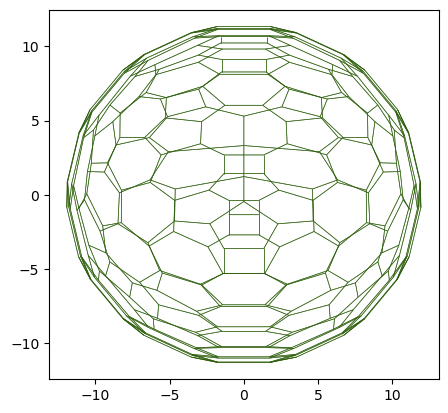
Closed sheet in 2.5D

For closed surfaces, a ClosedSheetGeometry is available. Calling update_all computes the enclosed volume of the sheet, and stores it the settings attribute as "lumen_vol"

from tyssue.geometry.sheet_geometry import ClosedSheetGeometry
from tyssue.generation import ellipsoid_sheet

ellipso = ellipsoid_sheet(a=12, b=12, c=21, n_zs=12)
ClosedSheetGeometry.update_all(ellipso)

lumen_vol = ellipso.settings['lumen_vol']

print(f"Lumen volume: {lumen_vol: .0f}")

Lumen volume:  11440

fig, (ax0, ax1) = plt.subplots(1, 2)

fig, ax0 = sheet_view(
    ellipso, 
    coords=["z", "y"],
    ax=ax0
)
fig, ax1 = sheet_view(
    ellipso, 
    coords=["x", "y"],
    ax=ax1
)

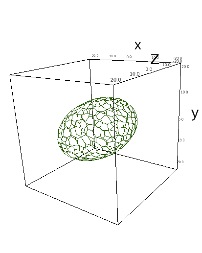
sheet_view can be called in 3D mode with ipyvolume:

import ipyvolume as ipv
ipv.clear()
fig, mesh = sheet_view(ellipso, mode="3D")
fig

---------------------------------------------------------------------------
ModuleNotFoundError                       Traceback (most recent call last)
Cell In[18], line 1
----> 1 import ipyvolume as ipv
      2 ipv.clear()
      3 fig, mesh = sheet_view(ellipso, mode="3D")

File ~/checkouts/readthedocs.org/user_builds/tyssue/conda/latest/lib/python3.12/site-packages/ipyvolume/__init__.py:8
      6 from ipyvolume import datasets  # noqa: F401
      7 from ipyvolume import embed  # noqa: F401
----> 8 from ipyvolume.widgets import *  # noqa: F401, F403
      9 from ipyvolume.transferfunction import *  # noqa: F401, F403
     10 from ipyvolume.pylab import *  # noqa: F401, F403

File ~/checkouts/readthedocs.org/user_builds/tyssue/conda/latest/lib/python3.12/site-packages/ipyvolume/widgets.py:23
     21 import ipyvolume._version
     22 from ipyvolume.traittypes import Image
---> 23 from ipyvolume.serialize import (
     24     array_cube_tile_serialization,
     25     array_serialization,
     26     array_sequence_serialization,
     27     color_serialization,
     28     texture_serialization,
     29 )
     30 from ipyvolume.transferfunction import TransferFunction
     31 from ipyvolume.utils import debounced, grid_slice, reduce_size

File ~/checkouts/readthedocs.org/user_builds/tyssue/conda/latest/lib/python3.12/site-packages/ipyvolume/serialize.py:17
     15 import ipywidgets
     16 import ipywebrtc
---> 17 from ipython_genutils.py3compat import string_types
     19 from ipyvolume import utils
     22 logger = logging.getLogger("ipyvolume")

ModuleNotFoundError: No module named 'ipython_genutils'

Monolayer

To represent monolayers, we add a cell element and dataframe to the datasets.

One easy way to create a monolayer is to extrude it from a sheet, that means duplicating the 2D mesh to represent the basal surface and linking both meshes together to form lateral faces.

from tyssue import Monolayer, MonolayerGeometry, ClosedMonolayerGeometry
from tyssue.generation import extrude

extruded = extrude(sheet_3d.datasets, method='translation')
specs = config.geometry.bulk_spec()
monolayer = Monolayer('mono', extruded, specs)
MonolayerGeometry.update_all(monolayer)
MonolayerGeometry.center(monolayer)

monolayer.cell_df.head()

	x	y	z	is_alive	area	vol	num_faces	id	num_ridges
cell
0	1.125000	1.250000	-0.5	1	4.118034	0.5000	6	0	24
1	2.000000	1.125000	-0.5	1	5.368034	0.8750	7	0	30
2	3.000000	1.125000	-0.5	1	5.368034	0.8750	7	0	30
3	4.000000	1.125000	-0.5	1	5.368034	0.8750	7	0	30
4	4.666667	1.208333	-0.5	1	2.802051	0.1875	5	0	18

In cell_df, the num_faces is self-explanatory, and the num_ridges the number of half_edges on the face.

Similarly to edges, in 3D each face is a “half face”, i.e. the interface between two cells consists of two faces, one per cell.

ipv.clear()
fig, mesh = sheet_view(monolayer, mode="3D")
fig

Faces and edges in a monolayer belong to a segment: apical, basal or lateral.

monolayer.face_df["segment"].unique()

array(['apical', 'basal', 'lateral'], dtype=object)

We can filter the data based on these segments:

apical_faces = monolayer.face_df[
    monolayer.face_df["segment"] == "apical"
]

It is possible to extract the basal or apical sheets from a monolayer with monolayer.get_sub_sheet:

basal = monolayer.get_sub_sheet("basal")

fig, ax = sheet_view(basal, coords=['x', 'y'], edge={"head_width": 0.1})

(Notice the basal sheet is oriented downward).

Closed Monolayer

Similarly to sheet, monolayers can be closed with a defined lumen.

datasets = extrude(ellipso.datasets, method='homotecy', scale=0.9)

mono_ellipso = Monolayer('mono_ell', datasets)
mono_ellipso.vert_df['z'] += 5

ClosedMonolayerGeometry.update_all(mono_ellipso)

ipv.clear()

fig, mesh = sheet_view(mono_ellipso, mode="3D")
fig

mono_ellipso.settings

{'lumen_vol': 8344.553887776496}

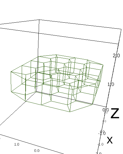
Bulk tissue

Eventually, we can define arbitrary assemblies of cells.

A way to generate such a tissue is through 3D Voronoi tessalation:

from tyssue import Epithelium, BulkGeometry
from tyssue.generation import from_3d_voronoi, hexa_grid3d
from tyssue.draw import highlight_cells
from scipy.spatial import Voronoi

cells = hexa_grid3d(4, 4, 6)
datasets = from_3d_voronoi(Voronoi(cells))
bulk = Epithelium('bulk', datasets)
bulk.reset_topo()
bulk.reset_index(order=True)
bulk.sanitize()

BulkGeometry.update_all(bulk)

# We'll see next how to configure visualisation

bulk.face_df['visible'] = False

highlight_cells(bulk, [12, 4])
ipv.clear()
fig2, mesh = sheet_view(bulk, mode="3D",
                        face={"visible":True})
fig2

Advanced example: better initial cells

Due to artifacts in the Voronoï tessalation at the boundaries of the above epithelium, the cells are ugly, with vertices protruding away from the tissue.

Here we show how to bring the vertices too far from the cell at a closer distance to the cells.

This will be the occasion to apply “upcasting” and “downcasting”.

Our algorithm is simple: for each vertex belonging to only one cell1, bring the vertex at a distance equal to the median cell-vertex distance towards the cell. Here is a 2D illustration:

Step 1. get the vertices that belong to a single cell

edge_df stores the topology of the tissue. We can use Apply / Groupby strategies to get vertices with only one cell:

bulk.vert_df['num_cells'] = bulk.edge_df.groupby("srce").apply(lambda df: df['cell'].unique().size)
bulk.vert_df['num_cells'].head()

vert
0    3
1    1
2    1
3    2
4    1
Name: num_cells, dtype: int64

Step 2. Create a binary mask over vertices with only one neighbor cell

lonely_vs = bulk.vert_df['num_cells'] < 2

Step 3. For each source vertex, compute the vector from cell center to the vertex, its length, and the median distance

rel_pos = bulk.edge_df[['sx', 'sy', 'sz']].to_numpy() - bulk.edge_df[['cx', 'cy', 'cz']].to_numpy()
    
rel_dist = np.linalg.norm(rel_pos, axis=1)
med_dist = np.median(rel_dist)

The displacement we need to apply is parallel to the cell-to-vertex vector, and can be expressed as:

displacement = rel_pos * (med_dist / rel_dist - 1)[:, np.newaxis]

We use np.newaxis to multiply 2D arrays of shape (Ne, 3) with 1D arrays of shape (Ne,).

This is still defined for each edge source.

We can come back to vertices by taking the mean over all outgoing edges:

# create a df so we can groupby
displacement = pd.DataFrame(displacement, index=bulk.edge_df.index)
displacement['srce'] = bulk.edge_df['srce']
vert_displacement = displacement.groupby("srce").mean()

Now we filter this with lonely_vs:

vert_displacement[~lonely_vs] = 0

Apply the displacement and update the geometry:

bulk.vert_df[['x', 'y', 'z']] += vert_displacement.to_numpy()

BulkGeometry.update_all(bulk)
ipv.clear()
fig2, mesh = sheet_view(bulk, mode="3D",
                        face={"visible":True})
fig2

---

1

This is not strictly necessary, we could do this for all the vertices, but it makes for an interesting example of filtering.