import numpy as np
import pandas as pd
import matplotlib.pyplot as plt
%matplotlib inline
from IPython.display import Image
from tyssue import config, Sheet, SheetGeometry, History, EventManager
from tyssue.draw import sheet_view
from tyssue.generation import three_faces_sheet
from tyssue.draw.plt_draw import plot_forces
from tyssue.dynamics import PlanarModel
from tyssue.solvers.viscous import EulerSolver
from tyssue.draw.plt_draw import create_gif
geom = SheetGeometry
model = PlanarModel
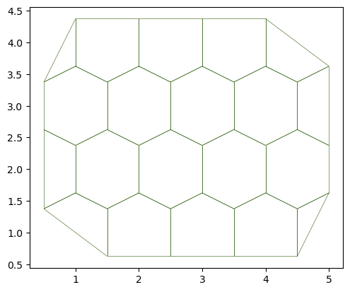
sheet = Sheet.planar_sheet_3d('planar', nx=6, ny=6,
distx=1, disty=1)
sheet.sanitize(trim_borders=True, order_edges=True)
geom.update_all(sheet)
fig, ax = sheet_view(sheet)
/tmp/ipykernel_3548/2598470357.py:2: DeprecationWarning:
Pyarrow will become a required dependency of pandas in the next major release of pandas (pandas 3.0),
(to allow more performant data types, such as the Arrow string type, and better interoperability with other libraries)
but was not found to be installed on your system.
If this would cause problems for you,
please provide us feedback at https://github.com/pandas-dev/pandas/issues/54466

  import pandas as pd
This module needs ipyvolume to work.
You can install it with:
$ conda install -c conda-forge ipyvolume
CGAL-based mesh generation utilities not found, you may need to install CGAL and build from source
C++ extensions are not available for this version
collision solver could not be imported You may need to install CGAL and re-install tyssue
The history object#
The History class defines the object in charge of storing the evolving epithelium during the course of the simulation. It allows to access to different time points of a simulation from one unique epithelium.
Most of the time, we use HistoryHDF5 class, that writes each time step to a file, which can be useful for big files. It is also possible to read an hf5 file to analyze a simulation later.
In the solver, we use the history.record method to store the epithelium.In the create_gif function, we use the history.retrieve method to get back the epithelium at a given time point. Please see the API for more details.
history = History(sheet, save_every=2, dt=1)

for i in range(10):

    geom.scale(sheet, 1.02, list('xy'))
    geom.update_all(sheet)
    # record only every `save_every` time
    history.record()

create_gif(history, 'simple_growth.gif', num_frames=len(history))


Image('simple_growth.gif')
retrieve returns an epithelium of the same type as the original:
type(history.retrieve(5))
tyssue.core.sheet.Sheet
Iterating over an history object yields a time and a sheet object:
for t, sheet in history:
    print(f"mean area at {t}: {sheet.face_df.area.mean():.3f}", )
mean area at 0.0: 0.781
mean area at 1.0: 0.813
mean area at 3.0: 0.880
mean area at 5.0: 0.952
mean area at 7.0: 1.031
mean area at 9.0: 1.116
The vert_h, edge_h and face_h DataFrames hold the history:
history.vert_h.head()
| vert | height | x | basal_shift | y | z | is_active | rho | time | |
|---|---|---|---|---|---|---|---|---|---|
| 0 | 0 | -4.0 | 0.5 | 4.0 | 2.625 | 0 | 1 | 0 | 0.0 |
| 1 | 1 | -4.0 | 1.5 | 4.0 | 3.375 | 0 | 1 | 0 | 0.0 |
| 2 | 2 | -4.0 | 2.5 | 4.0 | 2.625 | 0 | 1 | 0 | 0.0 |
| 3 | 3 | -4.0 | 0.5 | 4.0 | 3.375 | 0 | 1 | 0 | 0.0 |
| 4 | 4 | -4.0 | 1.0 | 4.0 | 3.625 | 0 | 1 | 0 | 0.0 |
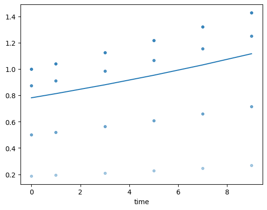
You can plot the evolution of a column vs time:
fig, ax = plt.subplots()

ax.scatter(history.face_h['time'], history.face_h['area'], alpha=0.2, s=12)

history.face_h.groupby('time').area.mean().plot(ax=ax)
<Axes: xlabel='time'>
Quasistatic solver#
A common way to describe an epithelium is with the quasistatic approximation: we assume that at any point in time, without exterior perturbation, the epithelium is at an energy minimum. For a given expression of the model’s Hamiltonian, we thus search the position of the vertices corresponding to the minimum of energy.
The Farhadifar model#
A very common formulation for the epithelium mechanical energy was given in Farhadifar et al. in 2007.
The energy is the sum of an area elasticity, a contractility and a line tension: $\( E = \sum_\alpha \frac{K_A}{2}(A_\alpha - A_0)^2 + \sum_\alpha \Gamma P_\alpha^2 + \sum_{ij} \Lambda \ell_{ij} \)$
This model has been predifined in tyssue as the default PlanarModel. We can use it in combination with a Solver object to find the energy minimum of our sheet.
To add the various columns in the dataframes (as we did above) we use a specification dictionnary with the required parameters.
#from tyssue.config.dynamics import quasistatic_plane_spec
from tyssue.dynamics.planar_vertex_model import PlanarModel as smodel
from tyssue.solvers import QSSolver
from pprint import pprint

specs = {
    'edge': {
        'is_active': 1,
        'line_tension': 0.12,
        'ux': 0.0,
        'uy': 0.0,
        'uz': 0.0
    },
   'face': {
       'area_elasticity': 1.0,
       'contractility': 0.04,
       'is_alive': 1,
       'prefered_area': 1.0},
   'settings': {
       'grad_norm_factor': 1.0,
       'nrj_norm_factor': 1.0
   },
   'vert': {
       'is_active': 1
   }
}


# Update the specs (adds / changes the values in the dataframes' columns)
sheet.update_specs(specs)

pprint(specs)
{'edge': {'is_active': 1,
          'line_tension': 0.12,
          'ux': 0.0,
          'uy': 0.0,
          'uz': 0.0},
 'face': {'area_elasticity': 1.0,
          'contractility': 0.04,
          'is_alive': 1,
          'prefered_area': 1.0},
 'settings': {'grad_norm_factor': 1.0, 'nrj_norm_factor': 1.0},
 'vert': {'is_active': 1}}
E_t = smodel.compute_energy(sheet)
print("Total energy: ", E_t)
Total energy: 13.44300213965199
smodel.compute_gradient(sheet).head()
| gx | gy | gz | |
|---|---|---|---|
| srce | |||
| 0 | -4.934718e-01 | -0.039296 | 0.0 |
| 1 | 0.000000e+00 | 0.163215 | 0.0 |
| 2 | -9.020562e-16 | -0.051386 | 0.0 |
| 3 | -3.863108e-01 | 0.021599 | 0.0 |
| 4 | -6.386835e-01 | 0.387129 | 0.0 |
The energy minimum is found with a gradient descent strategy, the vertices are displaced in the direction opposite to the spatial derivative of the energy. Actually, this defines the force on the vertices.
The gradient descent algorithm is provided by scipy minimize function, with the L-BFGSB method by default.
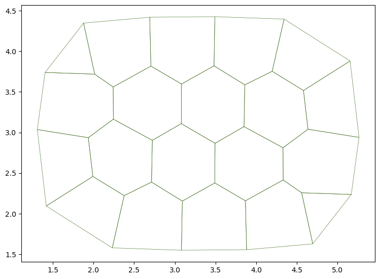
# Find energy minimum
solver = QSSolver()
res = solver.find_energy_min(sheet, geom, smodel)

print("Successfull gradient descent? ", res['success'])
fig, ax = sheet_view(sheet)

fig.set_size_inches(10, 10)
ax.set_aspect('equal')
Successfull gradient descent? True
Keyword arguments to find_energy_min method are passed to scipy’s minimize, so it is possible for example to reduce the termination criteria:
sheet.face_df.loc[4, "prefered_area"] = 2.0

res = solver.find_energy_min(sheet, geom, smodel, options={"ftol": 1e-2})
The method returns the output of the minimize function.
print("Boolean for the convergence success: ")
print(res.success)

print("Number of function evaluations: ")

print(res.nfev)

print("Information on the convergence: ")
print(res.message)
Boolean for the convergence success:
True
Number of function evaluations:
9
Information on the convergence:
CONVERGENCE: REL_REDUCTION_OF_F_<=_FACTR*EPSMCH
The solver object also provides facilities to approximate the gradient (can be useful when debugging new effectors) and evaluate the error between the actual gradient and the approximate one.
print('Total gradient error: ')
solver.check_grad(sheet, geom, model)
Total gradient error:
/home/docs/checkouts/readthedocs.org/user_builds/tyssue/conda/latest/lib/python3.12/site-packages/tyssue/solvers/base.py:19: FutureWarning: Setting an item of incompatible dtype is deprecated and will raise an error in a future version of pandas. Value '[1.49011612e-08 0.00000000e+00 0.00000000e+00 0.00000000e+00
 0.00000000e+00 0.00000000e+00 0.00000000e+00 0.00000000e+00
 0.00000000e+00 0.00000000e+00 0.00000000e+00 0.00000000e+00
 0.00000000e+00 0.00000000e+00 0.00000000e+00 0.00000000e+00
 0.00000000e+00 0.00000000e+00 0.00000000e+00 0.00000000e+00
 0.00000000e+00 0.00000000e+00 0.00000000e+00 0.00000000e+00
 0.00000000e+00 0.00000000e+00 0.00000000e+00 0.00000000e+00
 0.00000000e+00 0.00000000e+00 0.00000000e+00 0.00000000e+00
 0.00000000e+00 0.00000000e+00 0.00000000e+00 0.00000000e+00
 0.00000000e+00 0.00000000e+00]' has dtype incompatible with int64, please explicitly cast to a compatible dtype first.
  eptm.vert_df.loc[eptm.vert_df.is_active.astype(bool), eptm.coords] = pos.reshape(
0.1454401985184563
app_grad = solver.approx_grad(sheet, geom, model)
app_grad = pd.DataFrame(app_grad.reshape((-1, 3)), columns=['gx', 'gy', 'gz'])
app_grad.head()
| gx | gy | gz | |
|---|---|---|---|
| 0 | -0.000146 | 0.000176 | 0.0 |
| 1 | -0.000592 | 0.000862 | 0.0 |
| 2 | 0.000279 | -0.001307 | 0.0 |
| 3 | -0.000261 | 0.000547 | 0.0 |
| 4 | -0.000371 | -0.000068 | 0.0 |
Euler solver#
This notebooks demonstrates usage of the time dependent solver EulerSolver in the simplest case where we solve
$\(\eta_i \frac{d\mathbf{r}_i}{dt} = \mathbf{F}_i = - \mathbf{\nabla}_i E\)$
The model is used in the same way as the quasistatic solver.
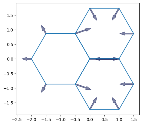
Simple forward Euler solver#
sheet = Sheet('3', *three_faces_sheet())
geom.update_all(sheet)
sheet.settings['threshold_length'] = 1e-3

sheet.update_specs(config.dynamics.quasistatic_plane_spec())
sheet.face_df["prefered_area"] = sheet.face_df["area"].mean()
history = History(sheet) #, extra_cols={"edge":["dx", "dy", "sx", "sy", "tx", "ty"]})

sheet.vert_df['viscosity'] = 1.0
sheet.edge_df.loc[[0, 17],  'line_tension'] *= 4
sheet.face_df.loc[1,  'prefered_area'] *= 1.2

fig, ax = plot_forces(sheet, geom, model, ['x', 'y'], 1)
Solver instanciation — contrary to the quasistatic solver, this solver needs the sheet, geometry and model at instanciation time:
solver = EulerSolver(
    sheet,
    geom,
    model,
    history=history,
    auto_reconnect=True)
The solver’s solve method accepts a on_topo_change function as argument. This function is executed each time a topology change occurs. Here, we reste the line tension to its original value.
def on_topo_change(sheet):
    print('Topology changed!\n')
    print("reseting tension")
    sheet.edge_df["line_tension"] = sheet.specs["edge"]["line_tension"]
Solving from \(t = 0\) to \(t = 15\)#
res = solver.solve(tf=15, dt=0.05, on_topo_change=on_topo_change,
                   topo_change_args=(solver.eptm,))
Topology changed!

reseting tension
Topology changed!

reseting tension
Showing the results#
create_gif(solver.history, "sheet3.gif", num_frames=120)
Image("sheet3.gif")