Dynamics

One of the objectives of tyssue is to make it easy to define and change the expression of the epithelium’s energy. For this, we define two classes of objects:

• Effector : those define a single energy term, evaluated on the mesh, and depending on the values in the dataframe. For example, line tension, for which the energy is proportional to the length of the half-edge, is defined as an Effector object (see bellow). For each effector, we define a way to compute the energy and its spatial derivative, the gradient.

• Model : a model is basically a collection of effectors, with the mechanisms to combine them to define the total dynamics of the system.

In general, the parameters of the models are addressable at the single element level. For example, the line tension can be set for each individual edge.

import sys
import pandas as pd
import numpy as np
import json
import matplotlib.pylab as plt
%matplotlib inline

from scipy import optimize

from tyssue import Sheet, config
from tyssue import SheetGeometry as geom
from tyssue.dynamics import effectors, model_factory
from tyssue.draw import sheet_view
from tyssue.draw.plt_draw import plot_forces
from tyssue.io import hdf5

/tmp/ipykernel_3509/3640356093.py:2: DeprecationWarning: 
Pyarrow will become a required dependency of pandas in the next major release of pandas (pandas 3.0),
(to allow more performant data types, such as the Arrow string type, and better interoperability with other libraries)
but was not found to be installed on your system.
If this would cause problems for you,
please provide us feedback at https://github.com/pandas-dev/pandas/issues/54466
        
  import pandas as pd

This module needs ipyvolume to work.
You can install it with:
$ conda install -c conda-forge ipyvolume

h5store = 'data/small_hexagonal.hf5'
#h5store = 'data/before_apoptosis.hf5'

datasets = hdf5.load_datasets(h5store)
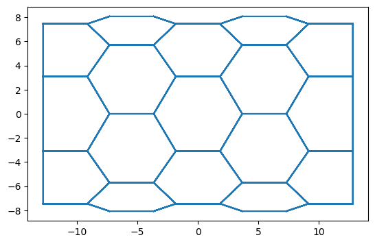
sheet = Sheet('emin', datasets)
sheet.sanitize(trim_borders=True, order_edges=True)

geom.update_all(sheet)

fig, ax = sheet_view(sheet, ['z', 'x'], mode='quick')

(Non)-Dimensionalization

If you read Farhadifar’s article or other modeling papers, you’ll see that the discussion on parameter values is done by defining unit dimensions, e.g. the unit length is defined such that the preferred area is unity. This can be done by defining dimension-less parameters and scaling them to correspond to the geometry (for example, line tension, which as units of energy per unit length, has a factor of \(\sqrt(A_0)\) between its dimension-less and its dimentionalized values. But in general it is simpler, and more robust computationally to scale the epithelium so that the average area is around unity (it is not strictly equivalent, but usually good enough), and then working with dimension-less units.

Comparison with the real tissue can then be done by homothetically scaling length to match e.g. average junction lengths between experiments and models.

geom.scale(sheet, 1/sheet.face_df['area'].mean()**0.5, coords=sheet.coords)
geom.update_all(sheet)

Effector classes

An effector designates a dynamical term in the epithelium governing equation. For quasistatic models, we need to provide a method to compute the energy associated with this effector, and the corresponding gradient.

For example, we can consider a line tension effector. The energy is \(E_t = \sum_{ij} \Lambda\ell_{ij}\) where the sum is over all the edges. For each half-edge, the gradient of \(E_t\) is defined by two terms, one for the gradient term associated with the half-edge \({ij}\) source, the over for it’s target. For the \(x\) coordinate: $\( \frac{\partial E_t}{\partial x_i} = \Lambda\left(\sum_k \frac{\partial \ell_{ik}}{\partial x_i} + \sum_m \frac{\partial \ell_{mi}}{\partial x_i}\right) = \Lambda\left(\sum_k \frac{x_i}{\ell_{ik}} - \sum_m \frac{x_i}{\ell_{mi}}\right) \)$

Where \(\sum_k\) is are over all the edges which vertex \(i\) is a source, and \(\sum_m\) over all the edges of which vertex i is a target.

Here is the definition of the line tension effector:

class LineTension(AbstractEffector):

    dimensions = units.line_tension
    magnitude = "line_tension"
    label = "Line tension"
    element = "edge"
    specs = {"edge": {"is_active": 1, "line_tension": 1e-2}}

    spatial_ref = "mean_length", units.length

    @staticmethod
    def energy(eptm):
        return eptm.edge_df.eval(
            "line_tension" "* is_active" "* length / 2"
        )  # accounts for half edges

    @staticmethod
    def gradient(eptm):
        grad_srce = -eptm.edge_df[eptm.ucoords] * to_nd(
            eptm.edge_df.eval("line_tension * is_active/2"), len(eptm.coords)
        )
        grad_srce.columns = ["g" + u for u in eptm.coords]
        grad_trgt = -grad_srce
        return grad_srce, grad_trgt

Predefined effectors

AbstractEffector : The abstract base class for all effectors

Edge effectors

LineTension : \(\Lambda \ell_{ij}\)

LengthElasticity : \(\frac{K_\ell}{2} (\ell_{ij} - \ell_0)^2\)

Face effectors

SurfaceTension : \(S A_{\alpha}\)

PerimeterElasticity : \(\frac{K_P}{2} (P_{\alpha} - P_0)^2\)

FaceAreaElasticity : \(\frac{K_a}{2} (a_{\alpha} - a_0)^2\)

FaceVolumeElasticity : \(\frac{K_v}{2} (V_{\alpha} - V_0)^2\) (Volume is computed with the “height” column of the face.

FaceContractility : \(\Gamma P_{\alpha}^2\)

Cell effectors

CellAreaElasticity : \(\frac{K_A}{2} (A_C - A_0)^2\)

CellVolumeElasticity : \(\frac{K_V}{2} (V_C - V_0)^2\)

Lumen effectors (for closed geometries)

LumenAreaElasticity : \(\frac{K_L}{2} (A_L - A_{L0})^2\)

LumenVolumeElasticity : \(\frac{K_L}{2} (V_L - V_{L0})^2\)

(There are some more in the effectors module but they are less generally useful)

Model factory

These effectors are then aggregated with others to define a model object. This object will have two methods compute_energy and compute_gradient that take an Epithelium object as single argument.

Such a model will usually be built with the function model_factory, that takes a list of effectors as input and returns a model object. For example, we can define the model from Farhadifar et al; by:

model = model_factory([
    effectors.LineTension,
    effectors.FaceContractility,
    effectors.FaceAreaElasticity
])

As for other aspects, the parameters are defined by a nested dictionary spec. Default values are gathered in the model.spec attribute:

model.specs

{'cell': {},
 'face': {'is_alive': 1,
  'perimeter': 1.0,
  'contractility': 1.0,
  'area': 1.0,
  'area_elasticity': 1.0,
  'prefered_area': 1.0},
 'edge': {'is_active': 1,
  'line_tension': 1.0,
  'sub_area': 0.16666666666666666},
 'vert': {},
 'settings': {'nrj_norm_factor': 1.0}}

We can use sheet.update_spec to set the correct columns in the sheet object.

Once the columns are set, it is possible to sets parameters for a subsets of edges (here by indexing the edges with a boolean series):

sheet.edge_df.loc[sheet.edge_df['sx']<0, 'line_tension'] = 0.5

sheet.update_specs(model.specs, reset=True)

Compute Energy

We now can compute the energy. By default, the compute_energy method returns a scalar, the total energy in the epithelium:

geom.update_all(sheet)
energy = model.compute_energy(sheet)
print(f'Total energy: {energy: .3f}')

Total energy:  364.185

We can compute all the energy terms with the full_output=True:

Et, Ec, Ea = model.compute_energy(sheet, full_output=True)

Et.head()

edge
0    0.323769
1    0.323769
2    0.322213
3    0.322213
4    0.322213
dtype: float64

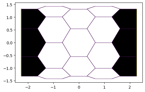
fig, ax = sheet_view(
    sheet,
    coords=list('zy'),
    face={"visible": True, "color": Ec, "colormap": "gray"},
    edge={"color": Et},
)

Computing the gradient

Similarly, by default, the gradient computes an array of shape (Nv, 3), with 3 coordinates (or 2 in 2D) for each vertex.

grad_E = model.compute_gradient(sheet)

grad_E.head()

	gx	gy	gz
srce
0	2.931605	1.214310e+00	-8.234192
1	2.931605	-1.214310e+00	-8.234192
2	2.640334	-1.093662e+00	-0.337580
3	2.892299	-1.040834e-14	-0.254173
4	2.640334	1.093662e+00	-0.337580

With components=True it returns a tuple of terms for each effector of the model.

gradients = model.compute_gradient(sheet, components=True)
gradients = {label: (srce, trgt) for label, (srce, trgt)
             in zip(model.labels, gradients)}
gradients['Line tension'][0].head()

	gx	gy	gz
edge
0	-0.00000	-0.000000	-0.500000
1	-0.00000	-0.000000	0.500000
2	0.08434	0.424007	0.251207
3	-0.08434	0.424007	-0.251207
4	0.08434	-0.424007	0.251207

Plotting forces

The tyssue.draw defines a useful plot_forces function:

fig, ax = plot_forces(sheet, geom, model, ['z', 'y'], scaling=0.1)
fig.set_size_inches(10, 12)

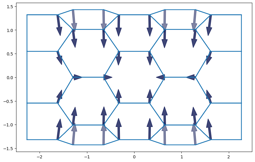
Fixing vertices

You may notice that the border vertices have no arrow. This is because they are not active, and do not participate in e.g. energy minimization, as we’ll see in the next section.