Energy minimization for a 2.5D sheet in 3D

import sys
import pandas as pd
import numpy as np
import json
import matplotlib.pylab as plt
%matplotlib inline

from scipy import optimize

from tyssue import Sheet

from tyssue import SheetGeometry as geom
from tyssue.dynamics.sheet_vertex_model import SheetModel as model 
from tyssue.solvers.quasistatic import QSSolver
from tyssue import config
from tyssue.solvers.isotropic_solver import bruteforce_isotropic_relax

from tyssue.draw.plt_draw import sheet_view
import tyssue.draw.plt_draw as draw
from tyssue.io import hdf5

/tmp/ipykernel_3741/3375153074.py:2: DeprecationWarning: 
Pyarrow will become a required dependency of pandas in the next major release of pandas (pandas 3.0),
(to allow more performant data types, such as the Arrow string type, and better interoperability with other libraries)
but was not found to be installed on your system.
If this would cause problems for you,
please provide us feedback at https://github.com/pandas-dev/pandas/issues/54466
        
  import pandas as pd

collision solver could not be imported You may need to install CGAL and re-install tyssue

This module needs ipyvolume to work.
You can install it with:
$ conda install -c conda-forge ipyvolume

h5store = 'data/small_hexagonal.hf5'

datasets = hdf5.load_datasets(h5store,
                              data_names=['face', 'vert', 'edge'])
specs = config.geometry.cylindrical_sheet()
sheet = Sheet('emin', datasets, specs)
sheet.sanitize(trim_borders=True, order_edges=True)

geom.update_all(sheet)
sheet.vert_df.describe().head(3)

	y	is_active	z	x	rho	old_idx	basal_shift	height	radial_tension
count	8.000000e+01	80.000000	8.000000e+01	8.000000e+01	8.000000e+01	80.000000	8.000000e+01	8.000000e+01	80.0
mean	1.110223e-15	0.800000	8.881784e-17	-2.620126e-15	8.071634e+00	103.425000	2.216705e+00	5.854929e+00	0.0
std	5.743517e+00	0.402524	8.027290e+00	5.743517e+00	4.968335e-15	27.759261	4.468911e-16	5.000389e-15	0.0

sheet.face_df.describe().head(3)

	area	z	y	is_alive	x	perimeter	old_idx	num_sides	vol	prefered_area	prefered_vol	contractility	vol_elasticity	prefered_height	basal_shift	basal_height	height	rho	id
count	40.000000	40.000000	4.000000e+01	40.0	4.000000e+01	40.000000	40.000000	40.000000	40.000000	40.0	40.0	40.000000	40.0	40.0	40.000000	40.000000	4.000000e+01	4.000000e+01	40.0
mean	31.948614	0.000000	1.176836e-15	1.0	-2.653433e-15	21.447238	27.500000	5.600000	187.056872	12.0	288.0	76.076404	1.0	24.0	2.500252	-3.246161	5.854929e+00	8.071634e+00	0.0
std	2.890942	7.446702	5.463498e+00	0.0	5.463498e+00	0.549335	16.306362	0.496139	16.926260	0.0	0.0	0.000000	0.0	0.0	0.000000	0.000000	2.491937e-15	2.257710e-15	0.0

sheet.edge_df.describe().head(3)

	dz	length	dx	dy	srce	trgt	face	old_jv0	old_jv1	old_cell	...	sz	tx	ty	tz	fx	fy	fz	rx	ry	rz
count	2.240000e+02	224.000000	2.240000e+02	2.240000e+02	224.000000	224.000000	224.000000	224.000000	224.000000	224.000000	...	224.000000	2.240000e+02	2.240000e+02	224.000000	2.240000e+02	2.240000e+02	224.000000	2.240000e+02	2.240000e+02	2.240000e+02
mean	3.965082e-18	3.829864	-1.982541e-17	-7.930164e-18	39.500000	39.500000	19.500000	99.348214	106.031250	27.500000	...	0.000000	-2.727977e-15	1.268826e-15	0.000000	-2.474211e-15	1.015061e-15	0.000000	3.965082e-17	-2.577303e-17	2.973812e-17
std	2.593865e+00	0.652700	2.053231e+00	2.053231e+00	23.111351	23.111351	11.563046	27.073959	27.627631	16.132856	...	7.530508	5.720290e+00	5.720290e+00	7.530508	5.409339e+00	5.409339e+00	7.117109	1.860313e+00	1.860313e+00	2.460756e+00

3 rows × 33 columns

Non dimensionalisation and isotropic model

For our 2D1/2 model, for a tissue energy is expressed as: $\( E = N_f\frac{K}{2}(V - V_0)^2 + N_f \frac{\Gamma}{2}L^2 + 3N_f\Lambda \ell \)\( In the case of a regular, infinite hexagonal lattice, There 6 edges per cell, each shared bteween 2 cells, hence \)Ne = 3N_f$

We can write this equation as a dimension-less one by dividing it by \(N_f K V_0^2\). We define the dimension-less values: \(\bar\Gamma = \Gamma/K V_0^{4/3}\) and \(\bar\Lambda = \Lambda/K V_0^{5/3}\)

\[ \bar{E} = \frac{\left(V/V_0 - 1\right)^2}{2} + \bar\Gamma \frac{V_0^{-2/3}}{2}L^2 + 3\bar\Lambda V_0^{-1/3} \ell \]

We define the scaling factor \(\delta\) such that \(V/V_0 = \delta^3\). On a regular hexagonal grid, the perimeter \(L=6\ell\) and the area is A=\(3\sqrt{3}/2\,\ell^2\). The volume is \(V = Ah\). As the (pseudo-)height is arbitrary, we can chose its prefered value. We set \(h_0 = V_0^{1/3}\).

We thus have \(A_0 = V_0^{2/3}\), \(A = \delta^2 V_0^{2/3}\) and \(\ell = \delta (\frac{2}{3\sqrt{3}})^{1/2} V_0^{1/3}\). We define the constant \(\mu = 2^{3/2}3^{1/4}\) to simplify further the equation:

\[\begin{split} \begin{eqnarray} \bar{E} &=& \frac{(\delta^3 - 1)^2}{2} + \frac{12}{\sqrt{3}}\bar\Gamma\delta^2 + \frac{6}{\sqrt{3}}\bar\Lambda \delta \\ \bar{E} &=& \frac{(\delta^3 - 1)^2}{2} + \frac{\mu^2}{2}\bar\Gamma\delta^2 + \frac{\mu}{2}\bar\Lambda \delta \\ \end{eqnarray} \end{split}\]

The root of this polynomial corresponds to the lowest energy possible for this set of paramters.

### This analytic model is implemented bellow

It is now a bit too specific to warrant a module in tyssue, and was thus removed

"""
Isotropic energy model from Farhadifar et al. 2007 article
"""
import numpy as np

mu = 2 ** 1.5 * 3 ** 0.25


def elasticity(delta):
    return (delta ** 3 - 1) ** 2 / 2.0


def contractility(delta, gamma):
    return gamma * mu ** 2 * delta ** 2 / 2.0


def tension(delta, lbda):
    return lbda * mu * delta / 2.0


def isotropic_energies(sheet, model, geom, deltas, nondim_specs):

    # bck_face_shift = sheet.face_df['basal_shift']
    # bck_vert_shift = sheet.vert_df['basal_shift']
    # ## Faces only area and height

    V_0 = sheet.specs["face"]["prefered_vol"]
    vol_avg = sheet.face_df[sheet.face_df["is_alive"] == 1].vol.mean()
    rho_avg = sheet.vert_df.rho.mean()

    # ## Set height and volume to height0 and V0
    delta_0 = (V_0 / vol_avg) ** (1 / 3)
    geom.scale(sheet, delta_0, sheet.coords)

    h_0 = V_0 ** (1 / 3)

    sheet.face_df["basal_shift"] = rho_avg * delta_0 - h_0
    sheet.vert_df["basal_shift"] = rho_avg * delta_0 - h_0
    geom.update_all(sheet)

    energies = np.zeros((deltas.size, 3))
    for n, delta in enumerate(deltas):
        geom.scale(sheet, delta, sheet.coords + ["basal_shift"])
        geom.update_all(sheet)
        Et, Ec, Ev = model.compute_energy(sheet, full_output=True)
        energies[n, :] = [Et.sum(), Ec.sum(), Ev.sum()]
        geom.scale(sheet, 1 / delta, sheet.coords + ["basal_shift"])
        geom.update_all(sheet)
    energies /= sheet.face_df["is_alive"].sum()
    isotropic_relax(sheet, nondim_specs)

    return energies


def isotropic_relax(sheet, nondim_specs, geom=geom):
    """Deforms the sheet so that the faces pseudo-volume is at their
    isotropic optimum (on average)
    The specified model specs is assumed to be non-dimentional
    """

    vol0 = sheet.face_df["prefered_vol"].mean()
    h_0 = vol0 ** (1 / 3)
    live_faces = sheet.face_df[sheet.face_df.is_alive == 1]
    vol_avg = live_faces.vol.mean()
    rho_avg = sheet.vert_df.rho.mean()

    # ## Set height and volume to height0 and vol0
    delta = (vol0 / vol_avg) ** (1 / 3)
    geom.scale(sheet, delta, coords=sheet.coords)
    sheet.face_df["basal_shift"] = rho_avg * delta - h_0
    sheet.vert_df["basal_shift"] = rho_avg * delta - h_0
    geom.update_all(sheet)

    # ## Optimal value for delta
    delta_o = find_grad_roots(nondim_specs)
    if not np.isfinite(delta_o):
        raise ValueError("invalid parameters values")
    sheet.delta_o = delta_o
    # ## Scaling
    geom.scale(sheet, delta_o, coords=sheet.coords + ["basal_shift"])
    geom.update_all(sheet)


def isotropic_energy(delta, mod_specs):
    """
    Computes the theoritical energy per face for the given
    parameters.
    """
    lbda = mod_specs["edge"]["line_tension"]
    gamma = mod_specs["face"]["contractility"]
    elasticity_ = (delta ** 3 - 1) ** 2 / 2.0
    contractility_ = gamma * mu ** 2 * delta ** 2 / 2.0
    tension_ = lbda * mu * delta / 2.0
    energy = elasticity_ + contractility_ + tension_
    return energy


def isotropic_grad_poly(mod_specs):
    lbda = mod_specs["edge"]["line_tension"]
    gamma = mod_specs["face"]["contractility"]

    grad_poly = [3, 0, 0, -3, mu ** 2 * gamma, mu * lbda / 2.0]
    return grad_poly


def isotropic_grad(mod_specs, delta):
    grad_poly = isotropic_grad_poly(mod_specs)
    return np.polyval(grad_poly, delta)


def find_grad_roots(mod_specs):
    poly = isotropic_grad_poly(mod_specs)
    roots = np.roots(poly)
    good_roots = np.real([r for r in roots if np.abs(r) == r])
    np.sort(good_roots)
    if len(good_roots) == 1:
        return good_roots
    elif len(good_roots) > 1:
        return good_roots[0]
    else:
        return np.nan

nondim_specs = config.dynamics.quasistatic_sheet_spec()
dim_model_specs = model.dimensionalize(nondim_specs)

sheet.update_specs(dim_model_specs, reset=True)
sheet.edge_df.is_active = (sheet.upcast_face(sheet.face_df.is_alive)
                           & sheet.upcast_srce(sheet.vert_df.is_active))
res = bruteforce_isotropic_relax(sheet, geom, model)

Et, Ec, Ev = model.compute_energy(sheet, full_output=True)
energy = model.compute_energy(sheet, full_output=False)
print('Total energy: {}'.format(energy))

Total energy: 18.662021831602555

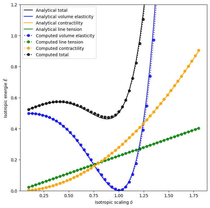
def plot_analytical_to_numeric_comp(sheet, model, geom, nondim_specs):

    fig, ax = plt.subplots(figsize=(8, 8))

    deltas = np.linspace(0.1, 1.8, 50)

    lbda = nondim_specs["edge"]["line_tension"]
    gamma = nondim_specs["face"]["contractility"]

    ax.plot(
        deltas,
        isotropic_energy(deltas, nondim_specs),
        "k-",
        label="Analytical total",
    )
    try:
        ax.plot(sheet.delta_o, isotropic_energy(sheet.delta_o, nondim_specs), "ro")
    except:
        pass
    ax.plot(deltas, elasticity(deltas), "b-", label="Analytical volume elasticity")
    ax.plot(
        deltas,
        contractility(deltas, gamma),
        color="orange",
        ls="-",
        label="Analytical contractility",
    )
    ax.plot(deltas, tension(deltas, lbda), "g-", label="Analytical line tension")

    ax.set_xlabel(r"Isotropic scaling $\delta$")
    ax.set_ylabel(r"Isotropic energie $\bar E$")

    energies = isotropic_energies(sheet, model, geom, deltas, nondim_specs)
    # energies = energies / norm
    ax.plot(
        deltas,
        energies[:, 2],
        "bo:",
        lw=2,
        alpha=0.8,
        label="Computed volume elasticity",
    )
    ax.plot(
        deltas, energies[:, 0], "go:", lw=2, alpha=0.8, label="Computed line tension"
    )
    ax.plot(
        deltas,
        energies[:, 1],
        ls=":",
        marker="o",
        color="orange",
        label="Computed contractility",
    )
    ax.plot(
        deltas, energies.sum(axis=1), "ko:", lw=2, alpha=0.8, label="Computed total"
    )

    ax.legend(loc="upper left", fontsize=10)
    ax.set_ylim(0, 1.2)
    print(sheet.delta_o, deltas[energies.sum(axis=1).argmin()])

    return fig, ax

fig, ax = plot_analytical_to_numeric_comp(sheet, model, geom, nondim_specs)

0.8865926873873902 0.8979591836734694

model.labels

['Line tension', 'Contractility', 'Volume elasticity']

gradients = model.compute_gradient(sheet, components=True)
gradients = {label: (srce, trgt) for label, (srce, trgt)
             in zip(model.labels, gradients)}
gradients['Line tension'][0].head()

	gx	gy	gz
edge
0	-0.000000	-0.000000	-668.132926
1	-0.000000	-0.000000	668.132926
2	112.700882	566.585593	335.679736
3	-112.700882	566.585593	-335.679736
4	112.700882	-566.585593	335.679736

grad_i = model.compute_gradient(sheet, components=False)
grad_i.head()

	gx	gy	gz
srce
0	-0.008983	-3.720720e-03	-0.001010
1	-0.008983	3.720720e-03	-0.001010
2	-0.018412	7.626655e-03	-0.009825
3	-0.013376	-7.264422e-17	-0.008121
4	-0.018412	-7.626655e-03	-0.009825

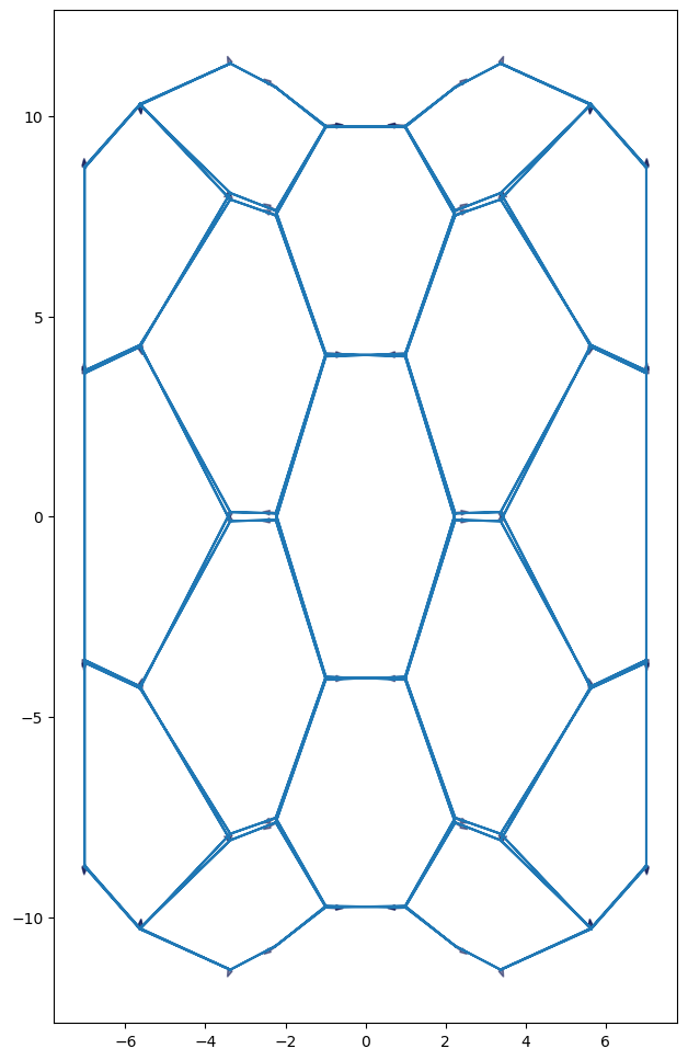
geom.scale(sheet, 1.2, sheet.coords)
geom.update_all(sheet)

scale = 5

fig, ax = draw.plot_forces(sheet, geom, model, ['z', 'x'], scale)
fig.set_size_inches(10, 12)
for n, (vx, vy, vz) in sheet.vert_df[sheet.coords].iterrows():
    shift = 0.6 * np.sign(vy)
    ax.text(vz+shift-0.3, vx, str(n))

app_grad_specs = config.draw.sheet_spec()['grad']
app_grad_specs.update({'color':'r'})

solver = QSSolver()    
sheet.topo_changed = False


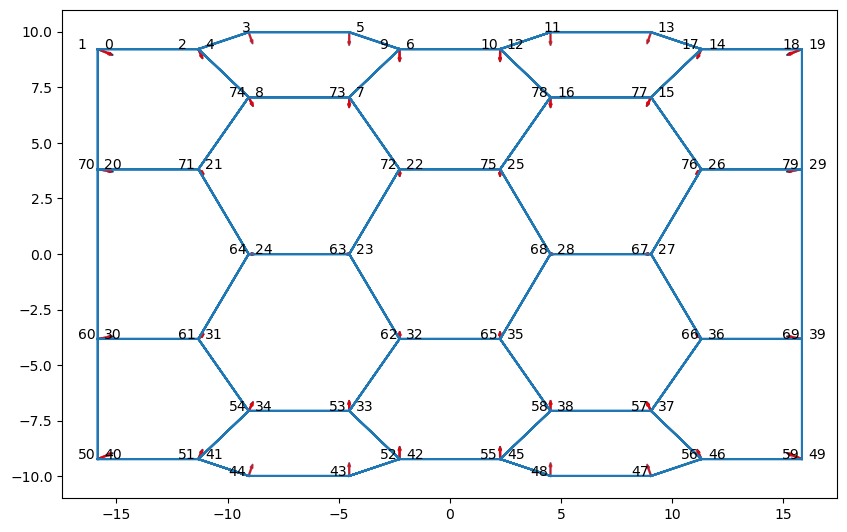
def draw_approx_force(ax=None):
    fig, ax = draw.plot_forces(sheet, geom, model,
                              ['z', 'x'], scaling=scale, ax=ax,
                              approx_grad=solver.approx_grad, **{'grad':app_grad_specs})
    fig.set_size_inches(10, 12)
    return fig, ax

## Uncomment bellow to recompute
fig, ax = draw_approx_force(ax=ax)
#fig

http://scipy.github.io/devdocs/generated/scipy.optimize.check_grad.html#scipy.optimize.check_grad

grad_err = solver.check_grad(sheet, geom, model)
grad_err /= sheet.Nv


print("Error on the gradient (non-dim, per vertex): {:.3e}".format(grad_err))

Error on the gradient (non-dim, per vertex): 1.688e-05

settings = {
        'options': {'disp':False,
                    'ftol':1e-5,
                    'gtol':1e-5},
        }


res = solver.find_energy_min(sheet, geom, model, **settings)
print(res['success'])

True

res['message']

'CONVERGENCE: REL_REDUCTION_OF_F_<=_FACTR*EPSMCH'

res['fun']/sheet.face_df.is_alive.sum()

0.43145767586018635

fig, ax = draw.plot_forces(sheet, geom, model, ['z', 'y'], 10)
fig.set_size_inches(10, 12)